Thanks to Will Hwang for his helpful thoughts and references on recent long context architectures.
A few weeks ago, DeepSeek released their V4 model, headlined by the tag: “Towards Highly Efficient Million-Token Context Intelligence”. Other models like Gemini and Claude have claimed million-token context before, but in practice were only effective for much shorter contexts on any real tasks. Deepseek V4 requires 27% of single-token inference FLOPs and 10% of KV cache that DeepSeek-V3.2 uses, which is already optimized for long-context tasks. These improvements have the community in astonishment (see below).
Keep getting rate-limited by Claude, so I tried out DeepSeek V4 for the first time.
— Jia-Bin Huang (@jbhuang0604) May 2, 2026
After 10M+ tokens, holy crap the cost is ... 🤯 pic.twitter.com/u5KfOCxv0X
I did a deep dive into the core architectural improvements which make such efficient processing of long contexts possible. There aren’t any detailed ablations in the paper, so we can only guess why they make these choices, but in my opinion, they are well motivated.
Surveying the land
Previous long-context architectures
The gold standard for long-context architectures, as far as I understand it, is hybrid architectures: interleaving layers of local attention, such as sliding window attention (SWA), or linear attention, like Gated DeltaNet, with layers of full attention, or global attention, at different ratios. Recency bias is a useful property in language as recent tokens are usually more relevant to the current query than older tokens, so we’re okay with this inductive bias. Fun fact: SWA was first proposed in 2020 with BERT models!Longformer: The Long-Document Transformer (Iz Beltagy et al, 2020) Talk about old.
For example, Gemma-3 has a 5:1 local-to-global ratio with SWA, meaning that there are 5 blocks of local attention followed by 1 block of global attention.Gemma 3 Technical Report (Team et al, 2025) With a local window of only 1024 tokens, this results in about $20\%$ of the KV cache that full attention in every layer would require. Kimi Linear instead features a 3:1 ratio of Gated DeltaNet style linear attention with full attention.Kimi Linear: An Expressive, Efficient Attention Architecture (Zhang et al, 2025)
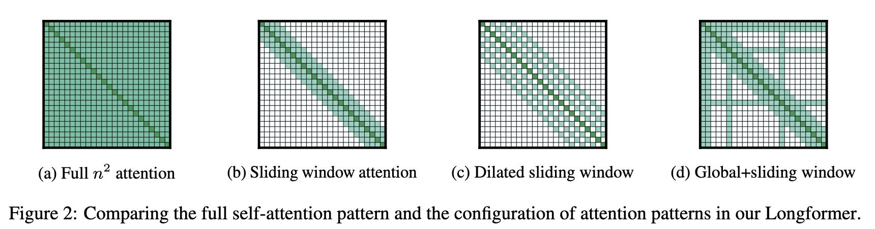
One of the first mentions of Sliding Window Attention (from Longformer).
This achieves a balance between speed/memory and explicit long context access in the KV cache. Note that SWA primarily tackles the memory explosion of the KV cache, and not any form of attention sharpening. Hybrid models still have a quadratic scaling factor, but the coefficient is much smaller, which tends to be good enough! Attempts to completely replace the quadratic factor with something sub-quadratic have not been very successful (see below).
One other issue with long context is that people tend to get cute with their attention mechanisms, which leads to theoretically interesting propositions. However, these patterns need to be hardware efficient to be useful in practice, so forms of sparse attention or global+sliding window are often slower despite their theoretical benefits. This is less of an issue in the modern day though, as people (AI) have gotten better at writing custom kernels.
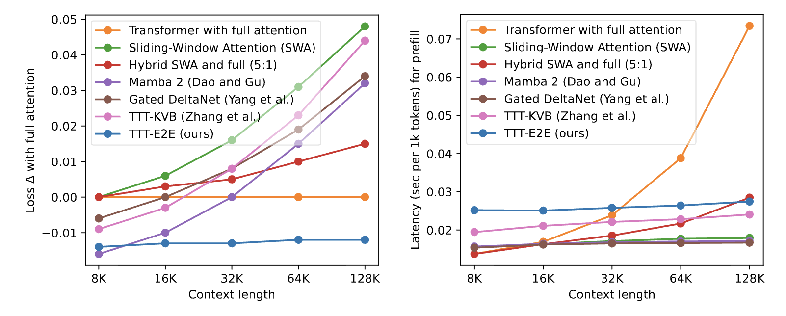
Comparison of different long-context architectures (from the E2E-TTT paper).
To prove my point above, this is a comparison of different long-context architectures from the E2E-TTT paper.End-to-End Test-Time Training for Long Context (Arnuv Tandon et al, 2025) Ignoring TTT-E2E (which is a still quite new), Hybrid SWA in the Gemma-3 ratio is the best performing loss at 128K context while also achieving a similar prefill latency to the other purported “long-context” methods. It’s a very strong baseline!
A wishlist for million-token context
Before we dive into DeepSeek V4’s specific architecture, let’s think about what the main inefficiencies with long context currently are.
Take a concrete use case: I’ve pasted an entire codebase into context and I want to know “where does the menu get repositioned on resize?” The repo has dozens of files spanning UI, backend, auth, and tests, but only two or three actually touch menu layout. The rest is dead weight that the model still has to pay attention over, token by token.
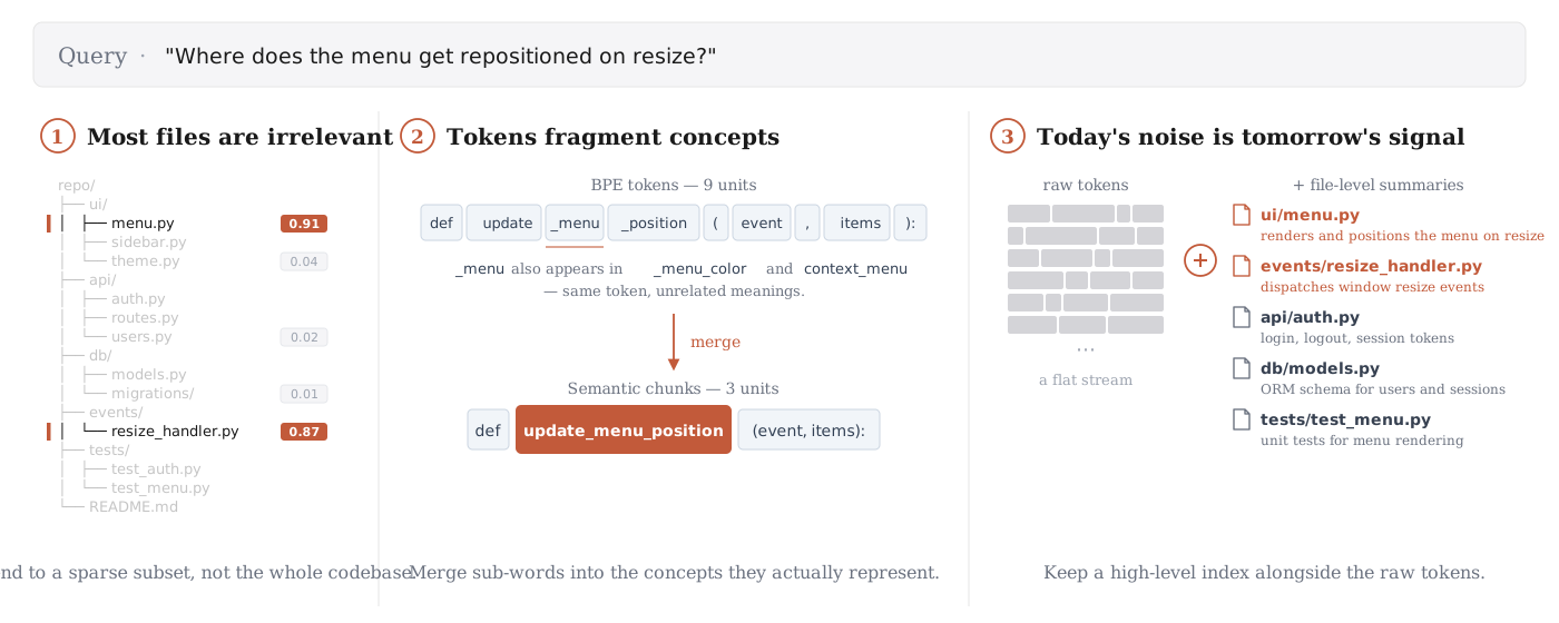
Three inefficiencies in long-context processing, illustrated on a single coding query. Thank you Claude.
This single example surfaces three distinct inefficiencies:
1. Most context is irrelevant. My UI code lives in a different directory than my auth or database code, and each makes up a small fraction of the total context. Spending compute attending over api/auth.py when the query is about menu positioning is wasted work. Worse, it dilutes attention away from the tokens that actually matter. Wishlist item #1: select a sparse set of the most relevant context.
2. Tokens are smaller than concepts. A real BPE tokenizer splits def update_menu_position(event, items): into roughly nine pieces — something like def, update, _menu, _position, (, event, ,, items, ):. The model sees update and _menu as separate units even though update_menu_position is the single concept that matches my query. _menu also shows up again in _menu_color, _menu_hidden, context_menu, so attention has to do extra work just to disambiguate the same subword across different uses. Wishlist item #2: merge tokens into higher-level concepts.
3. Noise now can be critical later. While we want a sparse context for each query, we also need a high level view of our entire context for our future queries.
If I follow up with “and how does login interact with the resize handler?”, api/auth.py suddenly matters and I need it back. Re-reading the full file from scratch every time the relevance landscape shifts is wasteful, so it would be much cheaper to keep a coarse representation of our entire context. Wishlist item #3: keep a coarse sketch of what you skipped.
Overview
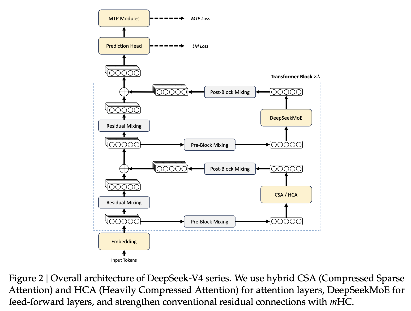
Overview of the DeepSeek-V4 Architecture.
The goal of DeepSeek-V4 is to achieve million-token context while maintaining the same level of performance as prior generations of models.DeepSeek-V4: Towards Highly Efficient Million-Token Context Intelligence (DeepSeek-AI, 2026) In this regime, the costly portion of the architecture is the attention mechanism, which scales quadratically with the context length, so the focus is entirely on reducing the KV cache size.
As we can see in the diagram above, DeepSeek features a hybrid architecture, interleaving a local Compressed Sparse Attention (CSA) with a global Heavily Compressed Attention (HCA) in a 1:1 ratio. There are other improvements, but most are either present in previous iterations of DeepSeek or aren’t as critical for long context.
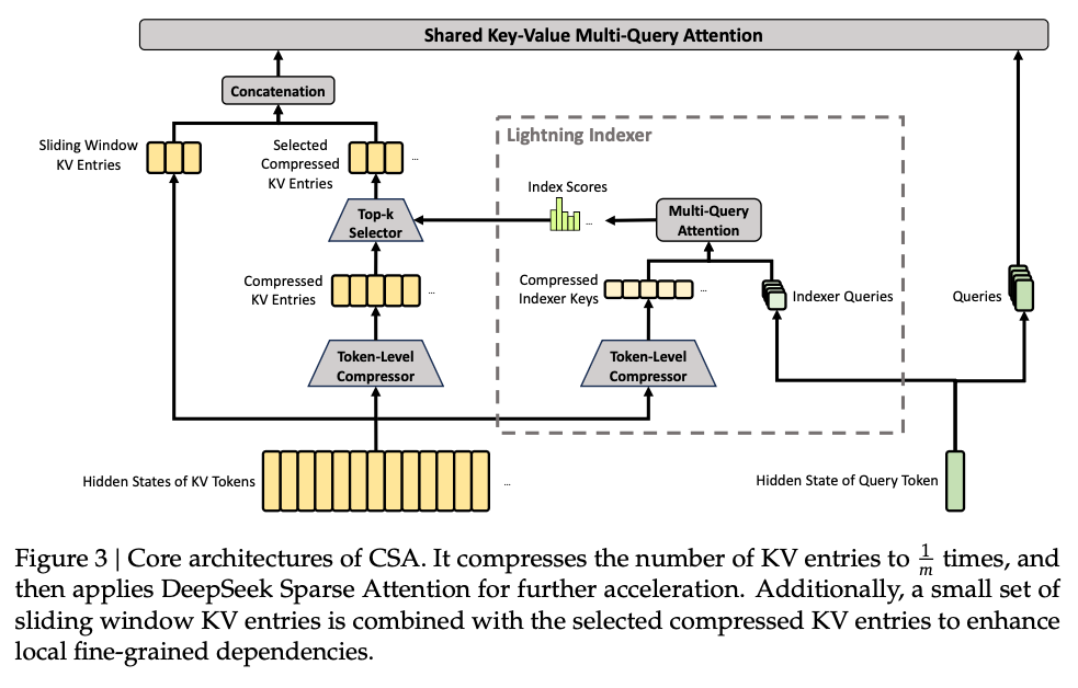
Compressed Sparse Attention (CSA) with DeepSeek Sparse Attention (DSA).
CSA tackles wishlist item #1: selecting a sparse set of the most relevant context. Each query token attends to only the most relevant $k$ compressed KV entries ($k = 128$). This is done with DeepSeek Sparse Attention (DSA) from DeepSeek-V3.2, using a Lightning Indexer to avoid the heavy $QK^T$ computation.
The “Compressed” part of CSA is done with a token-level compressor, which tackles wishlist item #2: merging tokens into higher-level concepts. It compresses every $m$ KV entries into $1$, so the model only attends over $\frac 1m$ as many entries ($m = 4$).
Finally, we can reuse the token-level compressor to perform Heavily Compressed Attention (HCA), which tackles wishlist item #3: keeping a coarse sketch of what you skipped. This compresses every $m' \gg m$ KV entries into $1$, a much more aggressive compression which aims to only keep the high level structure of the context ($m' = 128$).
We will now go through each of these components in detail.
Token-level compression
Our goal is to take an input hidden state $H\in \mathbb{R}^{n \times d}$ and reduce its sequence length by a factor of $m$, and optionally reduce its dimensionality to $c \ll d$. In other words, we want to bucket every $m$ tokens and compress them into a single token.
We’ll start with the simplest possible ideas and gradually fix their issues to get to the final solution.
First, let’s project our hidden state into a lower dimensional space:
$$ C = H W^{KV} \quad \text{where }\, W^{KV} \in \mathbb{R}^{d \times c} $$1. Average pooling with stride $(m, m)$
This is the simplest way to get from $m$ tokens to $1$ — average them together! Our compressed KV entries are then just
$$ C^{\text{comp}}_ i = \frac 1m \sum_{j=mi}^{m(i+1)-1} C_{j}.$$As expected, this sucks.
We’re losing so much information by blindly averaging info together as informative tokens get drowned out by noise. There’s a simple fix: learned weights.
2. Learnable weighted average
We should learn input-dependent weights for combining our tokens together. Let’s introduce a separate term for our compression weights:
$$ Z = HW^{Z} \quad \text{where }\, W^{Z} \in \mathbb{R}^{d \times c}.$$Now, we can compute weights using softmax just as we do in attention, so
$$ S_{mi: m(i+1) - 1} := \text{softmax}([Z_{mi: m(i+1) - 1}]) \implies C_i^{\text{comp}} = \sum_{j = mi}^{m(i+1)-1} S_j \odot C_j.$$However, now we have a slight issue: if my content spans across our window, we’ll be splitting the information up. So we should learn to integrate information across boundaries.
3. Boundary conditions
This only requires a simple fix: we simply need to integrate information from both the previous and current windows. We broaden our compression weights accordingly and sum across both windows.
$$ S_{{\color{red}m(i-1)}: m(i+1) - 1} := \text{softmax}([Z_{{\color{red}m(i-1)}: m(i+1) - 1}]) \implies C_i^{\text{comp}} = \sum_{j = {\color{red}m(i-1)}}^{m(i+1)-1} S_j \odot C_j.$$This has a tricky issue however, which is that there’s no positional nuance between when a window is acting as the current window to be compressed vs. as the context for the next window. Otherwise, we’ll be compressing the same information twice. This leads to our final solution.
4. Dual-role compression
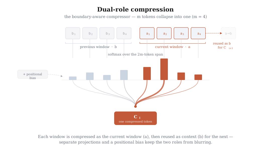
Thank you Claude for the visualization again.
To tackle this, we introduce a new set of weights for the previous window. Let $a$ refer to our current window, and $b$ refer to the previous window. Then we have four sets of states:
$$ \begin{aligned} \text{KV values:} &\quad C^a = H W^{aKV}, \quad C^b = HW^{bKV} \\ \text{KV compression weights:} &\quad Z^a = HW^{aZ}, \quad\,\;\; Z^b = HW^{bZ} \end{aligned} $$Let’s also introduce a learnable positional bias $\mathcal{B}^a, \mathcal{B}^b \in \mathbb{R}^{m \times c}$, which we’ll add to our KV compression weights to help further disambiguate context from current. This leaves us with
\[ [S^a_{mi: m(i+1) - 1}, S^b_{m(i-1): mi - 1}] = \text{softmax}([Z^a_{mi: m(i+1) - 1} + \mathcal{B}^a; Z^b_{m(i-1): mi - 1} + \mathcal{B}^b]). \]Then it remains to integrate this over our windows:
\[ C_i^{\text{comp}} = \sum_{j = mi}^{m(i+1)-1} S_j^a \odot C_j^a + \sum_{j = m(i-1)}^{mi-1} S_j^b \odot C_j^b \quad \in \mathbb{R}^{\frac nm \times c}. \]And we are done.
Remarks. I’m not personally sure of how important handling the boundary conditions is, but I’m assuming this is the primary motivation for DeepSeek’s implementation. There’s a lot of moving parts as well, and this softmax is slightly cheaper than attention (since we avoid the heavy $QK^T$ computation), so presumably this is worth the overhead for better representational power.
Compressed Sparse Attention (CSA)
Compressed Sparse Attention (CSA) uses the token-level compressor and the former DeepSeek Sparse Attention to select top-$k$ entries for the context. Thus, all we have left to explain is how the Lightning Indexer selects these entries.
First, we perform the same token-level compression as before to get compressed indexers $K^{\text{IComp}} \in \mathbb{R}^{\frac nm \times c^I}$, where $c^I \ll c$ is an even more compressed dimensionality than before $(c^I = 128)$. All we need from this is some idea of the relative importance of each indexer.
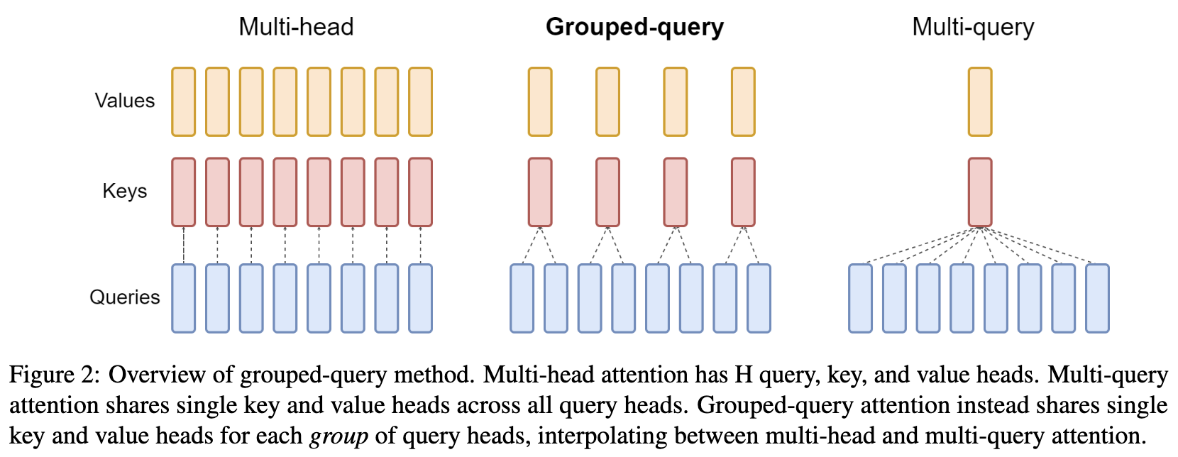
Multi-query attention (MQA) illlustration from the GQA paper.
To calculate the importance of each KV entry, we’re going to use multi-query attention (MQA).GQA: Training Generalized Multi-Query Transformer Models from Multi-Head Checkpoints (Joshua Ainslie et al, 2023) Unlike standard multi-head attention where we project our query, key, and value into $n_h$ different heads, we only project our query into different heads. This obviously comes at a cost of expressivity, but we don’t need much for index selection. We get the search power of 64 query heads, but we only have to store and fetch 1 Key head. This absolutely destroys the memory bandwidth bottleneck that normally plagues long-context decoding.
For a input token $t$ with hidden state $\mathbf{h}_t \in \mathbb{R}^d$, we produce multiple indexer queries $\{\mathbf{q}_{t,1}^I, \mathbf{q}_{t,2}^I, \ldots, \mathbf{q}_{t,n^I_h}^I\} \in \mathbb{R}^{n^I_h \times c^I}$ in a low-rank manner to save on compute.
$$ \underset{\substack{\\ \mathbb{R}^d}}{\mathbf{h}_t} \xrightarrow[\text{down-projection}]{W^{DQ}} \underset{\substack{\\ \mathbb{R}^{d_c} \\ \text{compressed latent} \\ \text{query vector}}}{\mathbf{c}_t^Q} \xrightarrow[\text{up-projection}]{W^{IUQ}} \underset{\substack{\\ \mathbb{R}^{c^I n_h^I}}}{\mathbf{q}_t^I} = \underbrace{\big[ \mathbf{q}_{t,1}^I ; \mathbf{q}_{t,2}^I ; \dots ; \overset{\in \mathbb{R}^{c^I}}{\mathbf{q}_{t,n_h^I}^I} \big]}_{n_h^I \text{ indexer query heads.}}. $$Here, we go from $d=4096$ to $d_c=1024$ as a downsample, to $n^I_h c^I=64\cdot 128 = 8192$ dimensions split between $n^I_h=64$ indexer query heads (which saves us ~50% compute compared to going directly). We also save on a factor of $n^I_h$ in our attention compared to if we had done standard multi-head attention, including the VRAM savings from having a much cheaper KV cache.
Finally, now that we have these queries and keys, we obtain the “values” for our multi-query attention (MQA) as
\[ [\mathbf{w}_{t,1}^I, \mathbf{w}_{t,2}^I, \ldots, \mathbf{w}_{t,n^I_h}^I] = \mathbf{w}^I_t = \mathbf{h}_t W^w \quad\quad W^w \in \mathbb{R}^{d \times n^I_h}.\]We use a cheap form of attention with ReLU as our nonlinearity instead of a softmax and sum over our query heads to obtain our final indexer scores:
\[ I_{t,s} = \sum_{h=1}^{n^I_h} \mathbf{w}_{t,h}^I \cdot \mathrm{ReLU}(\mathbf{q}_{t,h}^I\cdot K_{s}^{\text{IComp}}) \]where $s$ is the index of the preceding compressed block $(s \ll \lfloor \frac tm \rfloor)$. We take the top-$k$ compressed KV entries based on these scores, where $k=512$ for the Flash model.
Finally, while having compressed entries is good, we also maintain a sliding window of the most recent $n_{\text{win}}=128$ raw entries as well, as recent tokens are more relevant and still important to keep around.
Heavily Compressed Attention (HCA)
Heavily Compressed Attention is virtually the same as CSA, except we use a much more aggressive compression factor $m' \gg m$ to compress every $m'$ KV entries into $1$ ($m'=128$). This means we can also forgo the lightning indexer as the entire context is usually short enough to fit without needing sparsity.
Conclusion
DeepSeek V4’s architecture is a strong step towards million-token context. It maintains the hybrid design choice of its contemporary models, but is not quite as adventurous to use linear attention models like Gated DeltaNet.
I personally am excited to understand better why each choice was necessary (as there are no ablations), but the results clearly speak for themselves.
There’s some minor details about how RoPE needs to be applied in CSA that matter, but maybe I’ll save that for another day.
References
[1] Iz Beltagy, Matthew E. Peters, and Arman Cohan "Longformer: The Long-Document Transformer." arXiv:2004.05150 2020.
[2] Team, G., Kamath, A., Ferret, J., et al. "Gemma 3 Technical Report." 2025.
[3] Zhang, Y., Lin, Z., Yao, X., et al. "Kimi Linear: An Expressive, Efficient Attention Architecture." 2025.
[4] Arnuv Tandon, Karan Dalal, Xinhao Li, et al. "End-to-End Test-Time Training for Long Context." 2025.
[5] DeepSeek-AI "DeepSeek-V4: Towards Highly Efficient Million-Token Context Intelligence." 2026.
[6] Joshua Ainslie, James Lee-Thorp, Michiel de Jong, et al. "GQA: Training Generalized Multi-Query Transformer Models from Multi-Head Checkpoints." 2023.